This years OR 2014, the annual conference of the German Operations Research society, was hosted by our university, the RWTH Aachen during the first week of September. If you came to visit, I hope you had a wonderful time. One part of the entire conference organization was particularly interesting from the perspective of an optimizer. For any conference with multiple parallel streams it will be unavoidable that certain talks will be scheduled in parallel and can therefore not be attended at the same time. This means every attended will have to make the painful choice which talks she has to skip in favor of some other. The goal of a good schedule should therefore be to distribute the talks so that this pain is reduced. In the following I will give you some insight into how we modeled this problem in order to provide a great schedule for all our guests. The model presented here will be simplified in some respects - we took into account a whole bunch of details that are relevant for the conference but would make this article quite tedious to read.
This endeavor was not undertaken by me alone. My coworkers Michael Bastubbe, Sarah Kirchner und Markus Kruber where equally involved in this project.
Any model (and its results) can only be as good as the data we can feed in. So what data was available? For the talks we got some information from the EURO Online submission system (many thanks go to Bernard Fortz who helped us get this data):
- the title
- the abstract
- the list of keywords
- the list of authors
- the assigned session and stream
From this we basically saw only the keywords as a suitable way to derive the participants interest for a given talk. More fancy ways - trying to derive something from the abstracts by machine learning or other sources - were not feasible as we had no past data (who actually attended which talk in past conferences) to drive the learning. Therefore we asked the participants for their preferred keywords upon registration. This data was not mandatory - but provided by 646 participants when we calculated the schedule. Additionally we knew the times a participant had booked a tour. So we could make sure that no one had to give her talk while being on a tour.
Our objective was to keep the "pain" of choosing between talks low. The metric we had available for this was the match between a participants keywords and the keywords of a talk. As we did not want to account for session hopping (there should not be a need for that in a good plan) the smallest unit we had to schedule was a session. An easily available metric for how bad two sessions conflict might work as follows: For each pair of streams, sum up the number of keywords they share. Alternatively one could adjust this a little better and sum up the intersections between the keywords of the streams and those of each participant. Anyway this would lead us to a complete graph of all sessions, connected by edges which are weighted by some kind of measure how much those sessions conflict. Now a corresponding model might work by taking variables that encode if a session s is scheduled on timeslot t:
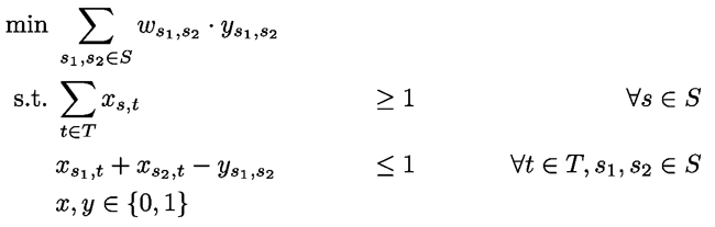
Here the first constraint makes sure that every session is scheduled and the second constraint enforces the penalty for two sessions that are scheduled in parallel. Note that I omitted a lot of details (room capacities and the like) to keep the focus on a single part of the problem.
This model turns out to be very bad. What do I mean with very bad? When put into a (state of the art) IP solver this produces a very bad LP relaxation - which means the solver is basically flying blind and cannot determine how good its current solution is. Furthermore a good LP relaxation often leads to better solutions found by the solvers primal heuristics.
Why is the LP relaxation of this model bad? To see this we need to go one step backwards. Given three specific sessions aligned in the following conflict graph:
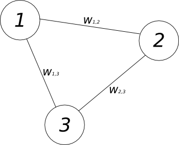
Now to make things even simpler let us only think about strict conflicts - so we forbid any of those sessions to share a timeslot. The constraints for this are:
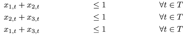
What is the issue with those constraints? A feasible (fractional) solution would be to assign a value of 0.5 to each variable. This way we could put a total of 1.5 session into a single timeslot. To avoid such "cheating" one can introduce an additional constraint, which combines the previous three:

These constraints (also known as clique cuts) are automatically added by a solver worth its salt (though one could help the solver if one happens to know large cliques in the conflict graph beforehand). This usually makes such scheduling problems with strict conflicts well solvable. This changes when we want to weaken the constraints like in our problem as the negative y terms destroy the structure that made the clique cuts possible. Therefore we decided to model the problem in a way that is directly more clique based.
When we look at a single participant, what she wants is, to have the sessions she likes distributed as evenly as possible. Given a session with 3 talks, each having 3 keywords, the most attractive sessions for her would have a match of 9 keywords. The worst case for her would be to have several such sessions scheduled in parallel. A little less bad would be to have several sessions in parallel, each having 8 of her favored keywords. And so forth. Based upon this we grouped sessions together into sets having 1 or more, 2 or more, …, up till 9 of the participants keywords. Each of these sets forms a clique which we can then penalize for appearing in the same timeslot. Note that for example a session with 9 matching keywords will appear in all 9 sets (and therefore gets a larger influence on the penalty). Counting the number of conflicting sessions per timeslot and set and adding those up per participant leads us to this model (where z carries the maximal amount of conflict for one participant and k is the number of shared keywords between a session and a participant):
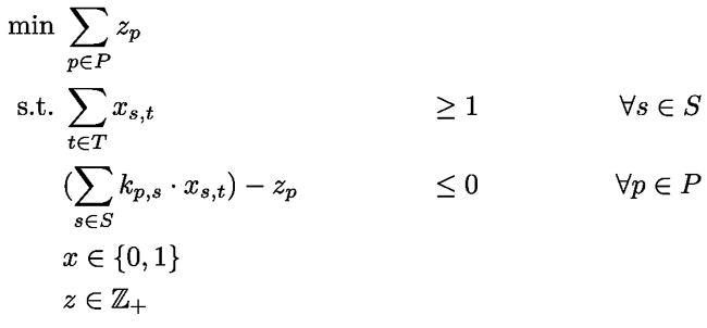
This formulation turns out to be much stronger - and leads to better solutions in less time. And with better I mean that they would have dominated the solutions (that where found within an hour) from the other model even compared to their objective function.
Lessons you can take away from this: If the objective is not an absolute (in this case there was no data to determine whether a certain objective would have been better than another) it makes sense to explore different models and go for one that works - until there is a need to change it. Also when modeling one should try to think "solver friendly". Formulations that are more clique based often turn out to perform better.
comments powered by Disqus