One or probably the most important algorithm in mathematical optimization is the Simplex method. Its origin dates back to the year 1947 when it was introduced by George Dantzig. It is the most widely used method to solve linear programming problems even though its worst case complexity is not polynomial and up till now no modification with this desired property is known. Despite this theoretical drawback it turns out that the simplex performs very well in practice and that it can be implemented to handle most real problems very well. In this post I will try to explain this popular algorithm in the way I currently understand it.
It all starts with some generic linear program:
A linear program describes some multidimensional polyhedron and we are looking for a point that maximizes a linear function which geometrically means that it is the furthest point into some specified direction. In 2D this could look as follows:
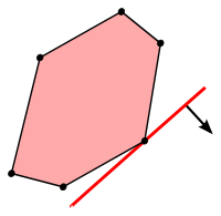
Despite this simplicity linear programs are very versatile and can describe a vast amount of problems, even though such models will likely have thousands of variables which prohibits us from imagining the resulting polytope.
Before we start to solve a linear program we need to first look at the properties of an optimal solution. For any constrained optimization problem (no matter if linear or not) there are two possibilities where an optimum can be: either it is somewhere inside the constraint region or it sits on its boundary. This insight is not very surprising. But given a linear objective we can quickly see that no optimal solution will be in the interior - it would be quite stupid to not go all the way along the direction of the objective. If even the constraints are linear (making the feasible region a polyhedron), we get the nice property that there will always be an optimal solution on one of the corners of the polyhedron. There may be other optimal points (one of the sides of the polyhedron could have the same angle as the objective) but one of them has to be on a corner.
The next insight is, that given we are on a corner of the polytope that is not an optimal one, there is one of the sides that we can walk along and improve the objective. This stems from the fact that our feasible region is convex:
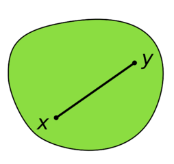
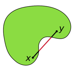
The idea is now to start in some corner of the polytope (it might not be easy to find that in the first place - but let us assume we found one lying around). Then go along some improving side until we can't anymore - and there we have our optimum.
How does this work in detail? First we need a way to describe the solution we have at hand. As it lies upon some of the constraints those constraints need to be satisfied with equality. Solving a system of linear equalities of the type
is straighforward if B is a square matrix and invertible. This means if we choose a certain number of variables and the same number of constraints to be fulfilled with equality, we can calculate some point lying on exactly those constraints using only the specified variables. The optimal solution has to specifiable in this way, we just don't know yet, which variables and constraints we should choose.
In order to simplify things one usually transforms the original problem to the following form
This formulation is completely equivalent, it just reformulates the inequalities by the introduction of the slack variables \(s\). The nice thing now is, that we only have equalities - with more variables than constraints. This should system of equalities therefore has many solutions. And such a solution is feasible, if no variable is negative. Given that we have \(m\) constraints we can specify a corner point of the polyhedron a choice of \(m\) of the variables - and then calculate this point by solving the linear system with the corresponding submatrix, which we call \(B\) (often denoted as basis). A chosen \(x\) variable will (if we disregard LP degeneracy) have a non zero value and a chosen slack variable corresponds to a constraint, upon which the specified corner will not be - due to the slack.
So now we have some feasible solution specified by the choice of our submatrix \(B\). What next? We need to check if there is some direction in which we can increase our objective value. To do so we need to know the "slope" (in direction of the objective) upon the constraints in the current corner into the directions of the variables which are currently not involved. Let \(N\) be the remaining part (not \(B\)) of \(A\) and \(I\). Also let \(c_B\) and \(c_N\) be the parts of the objective for the chosen or not chosen variables. This slope can then be calculated as
If any of these values is positive, that is a variable leading into an improving direction. That one should become part of \(B\). For it another one has to leave. It has to be chosen such that the resulting solution remains positive.
There likely are multiple choices for the entering and leaving variable. So many rules for choosing them (called pivoting rules) exist and it is still not known whether there exists a pivoting rule that leads the Simplex method to polynomial time performance in the worst case which would be huge break through.
Header photo by Death to the Stock Photo
comments powered by Disqus